MA1521-Notes

My take on MA1521 (AY23/24 Sem 1)

Definitions and concepts

1. Numbers

• Collection of real numbers R
• integers, rational no, irrational no. (not square root of negative no)
• closed interval [a,b] | open interval (a, b) | half-open intervals (a, b] or [a, b)

2. Absolute

• defined as a piecewise function |a| = { a, if a>=0 or -a, if a <0
• properties of |x|:
  • | − x| = |x|, for all x ∈ R.
  • |xy| = |x||y|, for all x,y ∈ R.
  • −|x| ≤ x ≤ |x|, for all x ∈ R.
  • For a fixed r > 0, |x| < r if and only if x ∈ (−r, r).
  • √x^2 = |x|, x ∈ R.
  • (Triangle Inequality) |x + y| ≤ |x| + |y| for all x,y ∈ R.

3. Functions

• f : A −→ B or a |→ f (a): a rule that assigns to each a ∈ A one specific member f (a) of B
• specify function -> gives rule f(x) = ....
• jargons
  • codomain: set B, the set of output the function is constrained to give
  • domain: set A, the set of values funciton f is being applied to
  • range: the subset of set B/codomain containing all the values of f -> range of f = {f (x) ∈ B | x ∈ A}
  • real-valued function (functions mapping to real numbers)
  • composite function: applying two functions to a value in succession, provided the first function's codomain matches the second function's domain: g ◦f : A → C given by g ◦ f (x) = g(f (x)).
  • inverse function f^-1: applying the two functions to a value x in succession in either order gives back value x
    • graph of inverse functions -> symmetric about y = x line
  • injective function: each x in the domain gives a unique output in the codomain after applying the function
  • surjective function: no z in B (codomain) is left alone -> every z in B has a corresponding x in A s.t. f(x) = z
  • bijective: injective and surjective

relations between domain, codomain, range.

4. Polynomials

• polynomial in degree n: a function in the form p(x) = anx^n + an-1x^n-1 + ... + a1x + a0, where an... are constants
• can be factored in as a product of linear and quadratic factors
• polynomial in degree n has at most n roots

5. Rational function

• function in the form of p(x)/q(x), where they are polynomials
• domain of it consists of all real numbers except the roots of q(x) -> division by zero error

6. Trigometric function

• sinx,cosx,tanx,cscx, secx,cotx
• periodic functions of period 2pi

7. Exponential and Logarithmic function

• f (x) = a^x, where a > 0
• logarithmic is inverse function of exponential: logax (to base a)
• e is Euler number, inverse of exponential function e^x is the natural logarithm lnx
• e^lnx = x for x > 0 and lne ^ x = x for all x
• domain of e^x is R and the range is the set R+ of all positive real numbers.

8. Domain and range in depth

• maximal domain: domain not specified -> take domain to be as large as possible (e.g. R \ {1})
• for some cases -> basic algebra can find the range of the function (let y = f(x) -> y = expr)

9. Limits

• let f be a real-valued function (R) defined on some interval I and c is a point in I
  • left limit: lim (x -> c-) f(x) is the value that f(x) approaches when x approaches c from the left.
  • right limit: lim(x -> c+) f(x) is the value that f(x) approached c from the right
  • let c be the interior point in I, if left limit = right limit = L (and L in R), lim(x -> c) f(x) exists and has value L
  • find limit from graph

10. Continuity and discontinuity

• discontinuity: hole, jump, infinite ~
• let f be a real-valued function (R) defined on some interval I and c is a point in I
  • if c is an interior point in I
  • f is continuous at c if (i) lim (x->c) f(x) exists and (ii) lim (x -> c)f(x) = f(c)
• c is the left end-point
  • f is continuous at x = c if (i) lim(x-> c+) f(x) exits and (ii) lim(x->c+) f(x) = f(c)
• c is the right end-point
  • f is continuous at x = c if (i) lim(x -> c-) f(x) exists and (ii) lim(x-> c-) f(x) = f(c)
• continuity on an interval: f is continuous on an interval if f is continuous at x = c for all points c in I.
• no sudden jump if continuous
• con and discon
• 3 steps con test

11. Evaluation of limits

• Laws of limits: (let L, M, c, and k be real numbers and lim(x->c)f(x) = L lim(x->c)g(x)=M
  1. Sum rule: + becomes L + M
  2. Difference rule: - becomes L - M
  3. Constant multiple rule: lim (x->c)(kf(x)) = kL
  4. Product rule: * becomes L * M
  5. Quotient rule: divide becomes L/M, M not equal 0
  6. Power rule: f(x) raised to the power of n becomes L^n, n is positive integer
  7. Root rule: f(x) root by n, becomes L root by n, n is a positive integer (or L^1/n)
• composite function limit: If g is continuous at the point b and lim(x→c)f (x) = b, then lim(x→c)g(f (x)) = g(b) = g(lim(x→c)f (x))).
• all these can be two-sided or one-sided limit, and the limit should exist
• Continuity of function implied by laws of limits:
  • If f and g are continuous at x = c, then for any constant k and any positive constant n, each of the following functions is continuous at x = c.
    • (i) f ± g, (ii) f^n, (iii) k* f , (iv) f g, (v) f /g provided g(c) not 0
  • If g is continuous at x = c and f is continuous at x = g(c), then the composite function f ◦ g is continuous at x = c.
• these functions are continuous on any interval contained on their maximal domain (PELT) :
  1. Polynomials
  2. Exponential functions
  3. Logarithmic functions
  4. Trigonometric functions
  5. Combination of any of the above on the domain it is defined
• Note: Since lim(x→c)f (x) = f (c) when f is continuous at x = c, finding the limit at x = c of any of the above functions is a matter of evaluating f at x = c.

12. Limits at infinity

• let f be dfined on R
  • lim(x-> ∞)f(x) is the value f(x) as x approaches positive infinity .
  • lim(x-> -∞)f(x) is the value f(x) as x tends to negative infinity.
• graphical representations if there is finite limit as x appraoches infinity -> asymptotes (horizontal, oblique...)
• asymptotes
  • A line y = b is a horizontal asymptote of the graph of a function y = ƒ(x) if either lim(x->∞)f(x) = b or lim(x->-∞)f(x) = b
  • A line x = a is a vertical asymptote of the graph of a function y = ƒ(x) if either lim(x->a+)f(x) = +-∞ or lim(x->a-)f(x) = +-∞
  • If the degree of the numerator of a rational function is 1 greater than the degree of the denominator, the graph has an oblique or slant line asymptote.
• dominant terms: a term in the expr dominates when x approaches const c/+∞/-∞ when it is large

13. Infinite limits, replacement rule

• indeterminate forms:
  • a limit of the form lim(x->c)(f(x)/g(x)) where f(x) -> 0 and g(x) -> 0 as x -> c is called an indeterminate form of the type 0/0
  • a limit of the form lim(x->c)(f(x)/g(x)) where f(x) -> ∞ and g(x) -> ∞ as x -> c is called an indeterminate form of the type ∞/∞
• replacement rule
  • Let I be an open interval containing the point x = c.Suppose f (x) = g(x) for all x ∈ I,except possibly at x = c, then lim(x->c)f(x) = lim(x->c)g(x)
  • this is useful when you encounter indeterminate forms and there exists a function g(x) to f(x) that are identical except at x =c, where f(x) is not defined but g(x) is well defined -> use the limit of g(x) at point c to find lim(x->c)f(x)
• theorem 12 in Thomos Calculas: all limits laws in Theorem 1 are true when we replace lim(x->c) by lim(x->∞) or lim(x->-∞); That is, the variable x may approach a finite number c or +-∞
• Note: lim(x->+-∞)(Ax^c + .../Bx^d + ...) -> which are the leading terms,
  • 0 if c < d
  • A/B if c = d
  • +-∞ if c > d
• useful results of tanx and sinx and tan(g(x)) and sin(g(x))

14. Squeeze (Sandwich) Theorem

Suppose g(x) ≤ f (x) ≤ h(x) for all x in some open interval containing a point c, except possibly at x = c. If lim(x->c)g(x) = lim(x->c)h(x) = L, then lim(x->c)f(x) = L

15. Intermediate Value Theorem (IVT)

If a real-valued function f is continuous on [a,b] and k is a number between f (a) and f (b),then f (c) = k for some c ∈ [a,b].

Deriavatives

1. slope of a curve y = ƒ(x) at the point P(x0, ƒ(x0)) AND deriavative of a function f at point x0

• is the number lim(h->0)( (f(x0 + h) - f(x0)) / h)
• provided the limit exists
• the tangent line to the curve at P is the line through P with this slope.

2. Deriavative of a function at point x

The derivative of the function ƒ(x) with respect to the variable x is the function ƒ′ whose value at x is lim(h->0)( (f(x + h) - f(x)) / h) provided the limit exists

• If ƒ′ exists at a particular x, we say that ƒ is differentiable (has a derivative) at x. If ƒ′ exists at every point in the domain of ƒ, we call ƒ differentiable
• alternative definition of derivative with z->x (let z = x + h)
• The process of calculating a derivative is called differentiation
• dy/dx means the deriative of y w.r.t. to x, not a ratio

3. Differentiable on an Interval; One-Sided Derivatives

A function y = ƒ(x) is differentiable on an open interval (finite or infinite) if it has a derivative at each point of the interval. It is differentiable on a closed interval [a, b4] if it is differentiable on the interior (a, b) and if the limits right-hand derivative at a and left-hand derivative at a

4. Differentiability Implies Continuity

If ƒ has a derivative at x = c, then ƒ is continuous at x = c.

5. Rules of differentiation

• Derivative of a Power: If n is a positive integer, then d/dx(x^n) = nx^(n-1 for all x where the powers xn and xn-1 are defined
• constant multiples: If u is a differentiable function of x, and c is a constant, then d/dx(cu) = c(du/dx)
• sum/difference rule: If u and y are differentiable functions of x, then their sum/difference u + y/ u - y is differentiable at every point where u and y are both differentiable. At such points, d/dx(u +- v) = du/dx +- dv/dx
• constant function: if f(x) has constant value ƒ(x) = c, then df/dx = d/dx(c) = 0
• product rule: If u and v are differentiable at x, then so is their product uv, and d/dx(uv) = vdu/dx + udv/dx
• quotient rule: If u and v are differentiable at x and if v(x) ≠ 0, then the quotient u/v is differentiable at x, and d/dx(u/v) = ( vdu/dx - udv/dx )/v^2

6. Second deriavative or higher order deriavative

• deriavatives of deriavatives

7. Deriavative as a rate of change

• The instantaneous rate of change of ƒ with respect to x at x0 is the derivative ƒ′(x0) = lim(h->0) (f(x0+h) - f(x0))/h

8. Velocity

Velocity (instantaneous velocity) is the derivative of position with respect to time. If a body’s position at time t is s = ƒ(t), then the body’s velocity at time t is v(t) = ds/dt = lim(change in t -> 0) (f(t+ change in t) - f(t)) / change in t

9. Speed

• speed measure the rate of progress rather than direction

Speed is the absolute value of velocity. Speed = |v(t)| = |ds/dt|

10. Acceleration

Acceleration is the derivative of velocity with respect to time. If a body’s position at time t is s = ƒ(t), then the body’s acceleration at time t is a(t) = dv/dt = d^2s/dt^2

• Jerk is the derivative of acceleration with respect to time: j(t) = da/dt = d^3s/dt^3

11. Deriavative of trigometric functions

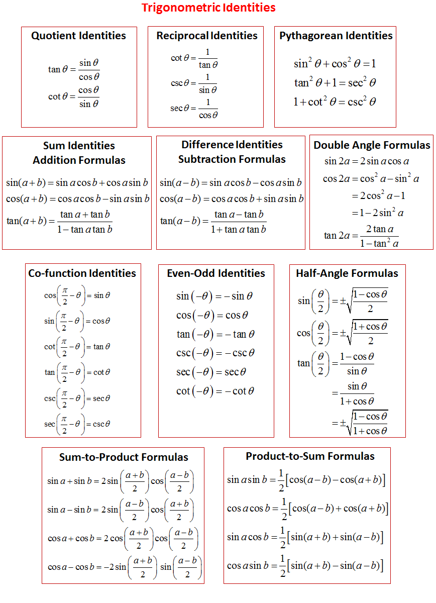
• angle sum formula
• d/dx(sin x) = cos x
• d/dx(cos x) = -sin x
• d/dx(tan x) = sec^2x
• d/dx(cot x) = -cosec^2 x
• d/dx(sec x) = sec x tan x
• d/dx(cosec x) = -cosec x cot x

12. The chain rule

• Thoerem 2

If ƒ(u) is differentiable at the point u = g(x) and g(x) is differentiable at x, then the composite function (ƒ ∘ g)(x) = ƒ(g(x)) is differentiable at x, and (ƒ ∘ g)′(x) = ƒ′(g(x)) * g′(x).

• In Leibniz’s notation, if y = ƒ(u) and u = g(x), then dy/dx = dy/du*du/dx (where dy/du is evaluated at u = g(x) )
• Inside-Outside rule
  • e.g. f(x) = sin(x^2 + x); f'(x) = cos (x^2 + x) * (2x + 1)
• chain rule with powers of a function
  • d/dx (u^n) = nu^(n-1) * du/dx

13. Implicit differentiation

y^n cases

• How:
  1. Differentiate both sides of the equation with respect to x, treating y as a dif�ferentiable function of x
  2. Collect the terms with dy>dx on one side of the equation and solve for dy>dx.
• differentiating deriavative of higher orders can think of substituting the result of dy/dx to the equation to make the final result consists of x and y only
• tangent (deriavative), normal (perpendicular, orthogonal)

14. Deriatives of Inverse Functions

• Bijectiveness
  • a bijective function (or one-one function) f has an inverse f−1 defined on the range of f
  • increasing or decreasing functions are bijective. (monotone functions) -> conclusive of injectivity
  • subjectivity is guranteed by the restriction of range (cover all y in the codomain)
  • f is increasing on I if x2 > x1 => f(x2) > f(x1) for all x1, x2 in I
  • f is decreasing on I if x2 > x1 => f(x2) < f(x1) for all x1, x2 in I
  • examples
  • e^x is increaseing on R (real numbers)
  • in x is increasing on R+ (or for x > 0)
  • if f and g are increasing on I then f+ g is increasing on I
  • if f is increasing or decreasing ten f has an inverse function f^-1
• Theorem 2.2
  • Let f be bijective and differentiable on an open interval I. Then (f^-1)'(a) = 1/(f'(f^-1(a)))
  • or = 1/f'(b)
  • or dx/dy = 1/(dy/dx) -> let y = y(x) be a function, suppose y has an inverse function x = x(y) then..

15. Higher order deriavative

• second deriavative of f, f'' or f^(2) superscript; provided that f' is differentiable: f''(x) = d/dx(('(x))
• In general, we can define the nth order derivative of f for any positive integer n provided the derivative exists.
• aka y'', D^2f(x)

16. Parametric equation

• a curve is defined by the parametric equation: x = f (t) and y = g(t), (t is the parameter)
• differentiable at a point where t = t0 if both f and g are differentiable at t = t0
• f'(t0) and g'(t0) not 0
• dy/dt = dy/dx * dx/dt => dy/dx = dy/dt / dx/dt = g'(t) / f'(t) (by chain rule)
• second deriavative -> replace y with dy/dx => d2y/dx2 = d/dt(dy/dx) / dx/dt = d/dt(g'(t)/f'(t)) / f'(t) = (g''(t)f'(t) - g'(t)f''(t)) / f'(t)^3
• examples of parametric curves
  • ellipses: (x - x0)^2/a^2 + (y - y0)^2/b^2 = 1
    • x = acost + x0; y = bsint + y0
  • hyperbolas: (difference: x less y)
    • x = asect + x0; y = btant + y0 OR x = atant + x0; y = bsect + y0
  • circles: (x-x0)^2 + (y - y0)^2 = r^2 (cartesian equation)
    • x = rcost + x0 and y = rsint + y0 (parametric equation) => search "How to convert from cartesian equation to parametric equation"
    • where r > 0, x0 and y0 are fixed constants and 0 <= t <= 2PI

17. Special forms

• deriavative of y = f(x)^g(x)
  • can be found by first finding the deriavative of ln y and then solving for dy/dx
• change of base formula
  • loga x = lnx/lna, a > 0 and a != 1

Application of deriavatives

solve optimisation problem easier

1. tangents and normal

• The tangent at the point (x0, f (x0)) on the graph of a differentiable function f has equation: y − f (x0) = m(x − x0)
• to check if parallel to axes
  • x axes: let dy/dx be 0
  • y axes: look at the deriavative of the normal (since normal is orthogonal to the tangent) (minus reciprocal of tangent)
• normal: gradient is m = f'(x0) (minus of the reciprocal)
• parametric equations: x = x(t) and y = y(t)
  • the equation of the tangent at the point where t = t0 is: y − y(t0) = m(x − x(t0))
  • the equation of the normal at the point where t = t0 is: y − y(t0) = −1/m(x − x(t0))
  • where m = dy/dx = dy/dt / dx/dt at t = t0

2. Absoulte maximum and min/ extremes/ global maxima or minima

Let ƒ be a function with domain D. Then ƒ has an absolute maximum value on D at a point c if f(x) <= f(c) for all x in D. and an absolute minimum value on D at c if f(x) >= f(c) for all x in D

3. Extreme value theorem (Theorem 3.4)

• If ƒ is continuous on a closed interval [a, b] , then ƒ attains both an absolute maximum value M and an absolute minimum value m in [a, b] . That is, there are numbers x1 and x2 in [a, b] with ƒ(x1) = m, ƒ(x2) = M, and m <= f(x) <= M for every other x in [a, b]
• only conclude existence but do not help us find the extreme value

4. Local maximum and minimum (Definition 3.5)

A function ƒ has a local maximum value at a point c within its domain D if ƒ(x) <= ƒ(c) for all x∊D lying in some open interval containing c. A function ƒ has a local minimum value at a point c within its domain D if f(x) >= f(c) for all x∊D lying in some open interval containing c.

• Theorem 3.8. (First Derivative Test for Local Extrema) Let f be differentiable on an open interval containing a critical point c except possibly at c and f is continuous at c.
  • (1) If f' changes from positive to negative at x = c, then f has a local maximum at c.
  • (2) If f' changes from negative to positive at x = c, then f has a local minimum at c
  • (3) If f' does not change sign at x = c, then f has no local extremum at c
• Theorem 3.9. (Second Derivative Test) Let f be a twice differentiable function defined in an open interval containing c.
  • (1) If f'(c) = 0 (horizontal tangent line) and f''(c) < 0 (concavity), then f has a local maximum at c.
  • (2) If f'(c) = 0 and f''(c) > 0, then f has a local minimum at c.
  • (3) No conclusion can be drawn if f''(c) = 0. (first deriavative test)
  • NOTE: The functions x^4, −x^4, x^3, has a local min, max, neither a max nor a min at x = 0, respectively, but have 0 second derivative at x = 0

5. Absolute extrema/global extrema (Definition 3.4)

A function f has an

• absolute maximum at x = c if f(x) <= f(c) for all x in the domain of f
• absolute minimum at x = c if f(x) >= f(c) for all x in the domain of f

• Theorem 3.7. (First Derivative Test for Absolute Extrema) Let f be differentiable on an open interval containing a critical point c except possibly at c and f is continuous at c.
  • (1) If f'(x) > 0 for all x < c and f'(x) < 0 for all x > c, then f has an absolute maximum at c.
  • (2) If f'(x) < 0 for all x < c and f'(x) > 0 for all x > c, then f has an absolute minimum at c.

7. The First Derivative Theorem for Local Extreme Values (THEOREM 2)

• If ƒ has a local maximum or minimum value at an interior point c of its domain, and if ƒ′ is defined at c, then ƒ′(c) = 0.
• Theorem 3.5. If f is differentiable on an open interval containing x = c and f has a local extremum at x = c, then f;(c) = 0.

7. interior point

An interior point of the domain of a function ƒ where ƒ′ is zero or undefined is a critical point of ƒ.

• to find absolute extrema of a continuous func f on a closed interval I
  • Find all critical points of ƒ on the interval.
  • Evaluate ƒ at all critical points and endpoints.
  • Take the largest and smallest of these values.
• (Critical Point Formal definition in LN) A number c in the domain of a function f is a critical point of f if the following 2 conditions hold
  1. it is not an end-point
  2. either f'(c) = 0 or f'(c) does not exist.
• Theorem 3.6. If f has a local minimum/maximum at x = c, then c is a critical point of f. (converse may not be true)

8. Rolle's Theorem (Theorem 3/ Theorem 3.11)

Suppose that y = ƒ(x) is continuous over the closed interval [a, b] and differentiable at every point of its interior (a, b). If ƒ(a) = ƒ(b), then there is at least one number c in (a, b) at which ƒ′(c) = 0.

• The hypotheses of Theorem 3 are essential. If they fail at even one point, the graph may not have a horizontal tangent.
• may be combined with the Intermediate Value Theorem to show when there is only one real solution of an equation ƒ(x) = 0

9. Mean Value Theorem (Theorem 4)

Suppose y = ƒ(x) is continuous over a closed interval [a, b] and differentiable on the interval’s interior (a, b). Then there is at least one point c in (a, b) at which (ƒ(b) - ƒ(a)) / (b - a) = ƒ′(c)

• physical interpretation: Mean Value Theorem says that the instantaneous change at some interior point is equal to the average change over the entire interval.
• colloary (mathematical consequences)
  • corollary 1: If ƒ′(x) = 0 at each point x of an open interval (a, b), then ƒ(x) = C for all x∊(a, b), where C is a constant.
  • corollary 2: If ƒ′(x) = g′(x) at each point x in an open interval (a, b), then there exists a constant C such that ƒ(x) = g(x) + C for all x∊(a, b). That is, ƒ - g is a constant function on (a, b).
• give us basis to use deriavative to find extrema
• consequence (collolary): Theorem 3.13. Let f be continuous on [a,b] and differentiable on (a,b). If f'(x) > 0(< 0) for all x ∈ (a,b), then f is increasing (decreasing) on [a,b]. (monotonocity)

10. Monotonic functions and first deriavative test

• to show that functions with postive deriavative is increasing function and that with negative deriavative is decreasing function: a function that is increasing or decreasing on an interval is said to be monotomic on an interval
• increasing and dereasing functions (definition in lecture notes)
  • collolary 3 (Theorem 3.1): Suppose that ƒ is continuous on [a, b] and differentiable on (a, b)
    • If ƒ′(x) > 0 at each point x∊(a, b), then ƒ is increasing on [a, b] (an interval I)
    • If ƒ′(x) < 0 at each point x∊(a, b), then ƒ is decreasing on [a, b]
  • first deriavative test for local extrema (218)
  • second deriavative test for local extrema (225)

11. Concavity

a graph of a differentiable function y = ƒ(x) is

• concave up on an open interval I if ƒ′ is increasing on I; (convex)
• concave down on an open interval I if ƒ′ is decreasing on I.
• The graph of f is concave upward (downward) on (a,b) if it is concave upward (downward) at every point in (a,b).

• second deriavative test for concavity
  • Let y = ƒ(x) be twice-differentiable on an interval I. (Theorem 3.2)
    • If ƒ″ > 0 on I, the graph of ƒ over I is concave up
    • If ƒ″ < 0 on I, the graph of ƒ over I is concave down

12. Points of inflection (Definition 3.3)

• A point (c, ƒ(c)) where the graph of a function has a tangent line and where the concavity changes is a point of inflection
  • At a point of inflection (c, ƒ(c)), either ƒ″(c) = 0 or ƒ″(c) fails to exist.
  • ^ (Theorem 3.3) . Let f be differentiable on (a,b). Let c ∈ (a,b). If (c, f (c)) is a point of inflection of the graph of f and f''(c) exists, then f''(c) = 0

13. Related rates

• let y = f(x) and let x and y be functions of a third var t that represents, e.g, time. By the chain rule, dy/dt = dy/dx*dx/dt

14. Maximum and Minimum Problem (Optimisation)

1. what is the var we want to maximise
2. find critical points (in the domain)
3. derivative test
4. conclude extrema

15. L'Hopital Rule

• Theorem 3.10. Let f and g be differentiable at all points in some open interval containing x = c (except possibly at c). If lim(x→c)f (x) = 0 = lim(x→c)g(x) or lim(x→c)f (x) = ∞ = lim(x→c)g(x), then
  • lim(x->c)f(x)/g(x) = lim(x->c)f'(x)/g'(x)
  • provided the limit on the right exists or equals ∞ or −∞.
  • The result also holds
    • (1) for limits at infinity, i.e. c = ±∞.
    • (2) for one-sided limits.
• three indeterminate forms: 0^0, infitity^0m 1^infinity

Integrals

1. Antideriatves

Definition 4.1. F is an antiderivative of f on an interval I if F'(x) = f (x) for all x in I.

• Theorem 4.1. (1) If F is an antiderivative of f on an interval I, then so is F + C for any constant C. Furthermore, any antiderivative of f on I is of the form F + C for some constant C. This can be expressed as
  • Int(f(x) dx) = F(x) + C
  • indefinite integral. (no range)
  • (2) Let α and β be any constants. Then int(αf (x) + βg(x)dx ) = αint(f (x)dx) + βint(g(x)dx)

2. Integration by substitution:

• Theorem 4.2. Let u = g(x) be a differentiable function whose range is some interval I and let f be continuous on I. Then, int(f(g(x))g'(x)dx) = int(f(u)du)
  • since u = g(x), we ave du/dx = g'(x). We may write du = g'(x)dx and then substitute f(g(x))g'(x)dx by f(u) du
  • theorem 4.3 -> right hand side also equal left hand side

3. Useful trignometrics identities for integration

• sec^2 x − 1 = tan^2 x
• csc^2 x − 1 = cot^2 x
• sinAcosA =1/2sin 2A
• cos^2 A =1/2(1 + cos 2A)
• sin^2 A =1/2(1 − cos 2A)
• sinAcosB =1/2(sin(A + B) + sin(A − B))
• cosAsinB =1/2(sin(A + B) − sin(A − B))
• cosAcosB =1/2(cos(A + B) + cos(A − B))
• sinAsinB = −1/2(cos(A + B) − cos(A − B))

4. Partial fractions (pg 71)

5. Integration by parts (pg 74)

• basic rule to determine which to differentate: LIATE (Log, Inverse trigo, Algebraic, Trigo, Exponential)

6. Riemann Sums and Definite Integrals

• divide the graph of f from x = a to b into n rectangles/ n equal distances (what happens when n approaches infinitiy? -> striaght lines, more dense, fill up entire area of the region; approximation better)
• without loss of generality -> area of a triangle = ( (b-a) / n) * f(a + k((b-a) / n) )
• grometrically: definite integral gives the area of the region uder the graph of f from x = a to x = b
  • int b/a (f(x) dx)
  • f must be continuous on [a,b]
• limit exists and is known as the definite integral of f from x = a to x = b

  • lim (n -> ∞) { sum (n k = 1)( (b-a) / n) * f(a + k((b-a) / n) )}

  • known as the Riemann sum of f -> sum (n k = 1)...
• for sufficiently large n,
  • int b a (f(x) dx) ≈ riemann sum
  • int is the limit of the riemann sum

7. Fundamental Theorem of Calculus (FTC) (79-80)

• riemann sum works but tedious
• First ~: Theorem 4.4 (FTC 1). Let f be continuous on [a,b] and let F be an anti-derivative of f .Then,
  • int b a (f(x) dx) = F(b) - F(a)
  • that is,
  • int b a(F'(x) fx) = F(b) - F(a)
  • often denoted by [F(x)]b a = F(b) - F(a)
  • FTC 1 follows from Theorem 4.5 (FTC 2)
• Second ~: Theorem 4.5 (FTC 2). Let f be continuous on [a,b]. The function g defined by g(x) = intx a (f(t) dt), a <= x <= b is continuous and differentiable on (a,b), and g'(x) = f(x). That is
  • d/dx (int x a (f(t) dt) ) = f(x)
  • essentially says that the area function int x a (f(t) dt) is an anti-deriavative of f
• useful remark: If g(x) is differentiable, then using the Chain Rule, one has d/dx( int g(x) a (f (t)dt) ) = f (g(x))g'(x).

8. Properties of definite integrals

• pg 83

9. Improper integral

Integrals with infinite limits of integration are improper integrals of Type I

1. f (x) is continuous on [a,∞): b is infinity --> lim (b ->∞ ) int b a (f(x) dx)
2. f (x) is continuous on (−∞,b]: a is -infinity --> lim (a ->-∞ ) int b a (f(x) dx)
3. f (x) is continuous on (−∞,∞): break into 2 parts to resemble step 1 and 2 (value c most of the cases are 0) --> equal parts; where c is any real number

• In each case, if the limit is finite, we say that the improper integral converges and that the limit is the value of the improper integral. If the limit fails to exist, then we say that the improper integral diverges.

Integrals of functions that become infinite at a point within the interval of integration are improper integrals of Type II.

1. f (x) is continuous on (a,b] and is discontinuous at a: replace a with c, then take limit of c, let it approach a from the right (c -> a+)
2. f (x) is continuous on [a,b) and is discontinuous at b: replace b with c, take limit of c, let it approach b from the left (c -> b-)
3. f (x) is discontinuous at c with a < c < b: break into two parts, and solve by parts using 1. and 2.

• In each case, if the limit is finite, we say that the improper integral converges and that the limit is the value of the improper integral. If the limit fails to exist, the improper integral diverges.

application of integration

1. Area between curves

• theorem 5.1: Let f and g be continuous on [a,b] with f (x) ≥ g(x) for all a ≤ x ≤ b. The area of the region bounded by the curves y = f (x),y = g(x), and the lines x = a and x = b is given by A = int b a( (f(x) - g(x))dx )
• Theorem 5.2. Let f be continuous on [a,b] with f (x) ≥ 0 for all a ≤ x ≤ b. The area of the region bounded by the curve y = f (x), the x-axis y = 0, and the lines x = a and x = b is given by A = int b a( f(x) dx )
  • when g(x) is 0, special case of the previous formula
• Theorem 5.3. Let f and g be continuous on [a,b] (not necessarily with f (x) ≥ g(x) for all a ≤ x ≤ b). The area of the region bounded by the curves y = f (x),y = g(x), and the lines x = a and x = b is given by A = int b a ( |f(x) - g(x)| dx)
  • more general case
  • To evaluate the above integral, we split it into two or more integrals, each corresponding to the region where either f (x) − g(x) ≥ 0 or f (x) − g(x) ≤ 0.
• Theorem 5.4. Let f be continuous on [a,b]. The area of the region bounded by the curve y = f (x), and the lines x = a and x = b is given by A = int b a( |f(x)| dx)
  • g(x) = 0 special case, the x-axis
  • To evaluate the above integral, we split it into two or more integrals, each corresponding to the region where either f (x) ≥ 0 or f (x) ≤ 0

can draw a graph to visualise the graph

• Theorem 5.5. Let f and g be continuous on [c, d] with f (y) ≥ g(y) for all c ≤ y ≤ d. The area of the region bounded by the curves x = f (y), x = g(y), and the lines y = c and y = d is given by A = int d c( (f(y) - g(y)) dy) - when it is easier for us to write the curves in terms of y (write x in terms of y))
• Theorem 5.6. Let f and g be continuous on [c, d] (not necessarily with f (y) ≥ g(y) for all c ≤ y ≤ d). The area of the region bounded by the curves x = f (y), x = g(y), and the lines y = c and y = d is given by A = int d c ( (|f(y) - g(y)|) dy)
  • general case when f(y) ≥ g(y) does not hold
  • To evaluate the above integral, we split it into two or more integrals, each corresponding to the region where either f (y) − g(y) ≥ 0 or f (y) − g(y) ≤ 0.

2. Volumn of Solid of Revolution by Disk (against x or y axis)

• Theorem 5.7. When the plane region bounded by the curve y = f (x) and the lines x = a and x = b is revolved completely about the x-axis, the volume of the solid formed is V = pi * int b a ( f(x)^2 dx)
  • disk method
• Theorem 5.8. Let f and g be continuous on [a,b] with f (x) ≥ g(x) ≥ 0 for all a ≤ x ≤ b. When the region bounded by the curves y = f (x) and y = g(x) for a ≤ x ≤ b is revolved completely about the x-axis, the volume of the solid formed is V = pi * int b a ( f(x)^2 dx) - pi * int b a( g(x)^2 dx)
• Theorem 5.9. Let f be continuous on [c, d]. When the plane region bounded by the curve x = f (y) and the lines y = c and y = d is revolved completely about the y-axis, the volume of the solid formed is V = pi * int d c( f(y) ^2 dy)
• Theorem 5.10. Let f and g be continuous on [c, d] with f (y) ≥ g(y) ≥ 0 for all c ≤ y ≤ d. When the region bounded by the curves x = f (y) and x = g(y) for c ≤ y ≤ d is revolved completely about the y-axis, the volume of the solid formed is V = pi * int d c( f(y) ^2 dy) - pi * int d c( g(y)^2 dy)

3. Cylindrical shell method

• When the plane region bounded by the curve y = f (x) and the lines x = a and x = b, where 0 ≤ a < b, is revolved completely about the y-axis, the volume of the solid formed is V = 2pi * int b a (x|f(x) dx)

4. Arc length of a curve

• Let f be continuous on [a,b]. Using Riemann sums, we can prove:
  • The length of the curve y = f (x),a ≤ x ≤ b is int b a ( sqrt(1 + f'(x)^2) dx ) --> horizontal curve
  • The length of the curve x = g(y), p ≤ y ≤ q is int b a( sqrt(1 + g'(y)^2) dy ) --> vertical curve
  • must note cases where y' is not well-defined at the interval
• math resource one
• khan

Sequences and series

positive integers vs real-valued function

1. Sequences

• Definition 6.1. An infinite sequence of numbers is a function whose domain is the set of positive integers. (then an is the value of the function eval at n) An infinite sequence of numbers is an infinite ordered list of numbers. a1, a2,...,an...

• usually denote a sequence by {an}∞/n = 1 or simply {an} when the reference to n is clear
• AP --> {a + (n-1)d}∞/n =1 and GP --> {ar^(n-1)}∞/n=1
• we want to find out what happens to an if n approaches infinity --> limit of a sequence
  • Let {an}∞/n=1 be a sequence of real numbers. Then lim(n→∞)an is the value an approaches as n tends to positive infinity.
  • If lim(n→∞)an exists as a real (finite) number L, then we say that the sequence {an} converges (or more detailedly, {an} converges to L). Sometimes we simply write an → L.
  • We say that the sequence {an} diverges if lim(n→∞)an does not exist as a real (finite) number.
    • either limit tends to infinity/ does not converge to any real numver e.g. {(-1)^n}

2. Finding the limit of a sequence

• Theorem 6.1. Let f (x) be a function, and {an} be a sequence such that f (n) = an for all n. If lim(x→∞)f (x) = L, then lim(n→∞)an = L.

3. Limit Laws for Sequences

• If {an} and {bn} are convergent sequences and c is a constant, then we have
  • lim(n→∞)c*an = c lim(n→∞)an.
  • lim(n→∞)(an ± bn) = lim(n→∞)an ± lim(n→∞)bn.
  • lim(n→∞)an*bn = lim(n→∞)an · lim(n→∞)bn.
  • lim(n→∞)an / bn=lim(n→∞)an / lim(n→∞)bn, if lim(n→∞)bn != 0.
• Theorem 6.2. (Squeeze Theorem for Sequence) If an ≤ bn ≤ cn for all n and lim(n→∞)an = lim(n→∞)cn = L, then lim(n→∞)bn = L.

4. Series

• An expression of the form sum ∞/n=1 an = a1 + a2 + a3 + a4 + ··· --> infite series or simply a series
• to compute the value (called sum) of this infinite series, we construct a new sequence [Sn] defined by Sn = sum n / i = 1 ai = a1 + a2 + ··· + an
  • [Sn] is called the sequence of partial sums of the given series
  • then the sum of the infinite series is defined as the limit of the sequence [Sn]
  • sum ∞ / n = 1 an = lim(n->∞)Sn
• we say that the series sum ∞ / n = 1 an converges if the sequence {Sn} converges (which means that lim(n→∞)Sn exists as a real number) --> thus the series is convergent means that it has a finite sum
• the series diverges if the partial sum diverges, is divergent means it does not have a finite sum (infinity/does not exist as a real number)
• GP --> sum ∞ / n =1 ar^(n-1) = a(r^n - 1)/r - 1
  • convergent when |r| < 1, and diverent if |r| >= 1
• can use differences of sum (learnt in JC)

Theorems:

• Theorem 6.3. If sum∞ / n=1 an and sum∞ / n=1 bn are convergent series, so are the series sum∞ / n=1 c*an (where c is a constant) and sum∞ /n=1 (an + bn). Moreover,
  1. sum∞ / n=1 c*an = c * sum∞ / n=1 an
  2. sum∞ / n=1 (an + bn) = sum∞ / n=1 an + sum∞ / n=1 bn
• Lemma 6.4. If the series sum∞ / n=1 an is convergent, then lim(n→∞)an = 0.
• Theorem 6.5. (The nth Term Test for Divergence):If lim(n→∞)an does not exist or if lim(n→∞)an != 0, then the series sum∞ / n=1 an is divergent.
  • note: ❗the nth term test is inconclusive if lim (n→∞)an = 0
• Theorem 6.6. A series sum∞ / n=1 an of nonnegative terms converges if and only if its partial sums are bounded from above (i.e., there exists a constant K such that Sn < K for all n.)
  • Basically, this theorem means that if each an ≥ 0, then the sum of the series sum∞ / n=1 an is either a finite number or ∞

5. Integral test

• a trick: see harmonic series (pg 113 in pdf)
• Theorem 6.7. (Integral Test) Let {an} be a sequence of positive terms. Suppose that an = f (n), where f is a continuous, positive, decreasing function of x for all x ≥ 1.
  • Then the series sum∞ / n=1 (an) is convergent if and only if the improper integral int ∞ 1(f (x)dx) is convergent.
  • (i) if int ∞ 1 (f(x) dx) is convergent, then sum ∞ / n = 1 (an) is convergent
  • (ii) if int ∞ 1 (f(x) dx) is divergent, then sum ∞ / n = 1 (an) is divergent
  • note: the result of the convergent integral (if exist) is not the sum of the series (is bigger)
• Theorem 6.8. (The p-series) The p-series sum ∞ / n=1 (1 / n^p) is convergent if and only if p > 1.

6. The comparison test

• Theorem 6.9. (Comparison Test): Suppose sum ∞ / n=1 an and sum ∞ / n=1 bn are series with nonnegative terms such that 0 ≤ an ≤ bn for all n.
  • (i) sum ∞ / n=1 bn is convergent, then sum ∞ / n=1 an is convergent
  • (ii) sum ∞ / n=1 an is divergent, then sum ∞ / n=1 bn is divergent
  • (i) means the bigger series has a finite sum, then the smaller series also has a finite sum
  • (ii) means that if the sum of the smaller series is ∞, then the sum of the bigger series is also ∞.
  • When applying the Comparison Test, we often compare a given series with an appropriate p-series or geometric series.

7. The ratio test and root test

• Theorem 6.10. (The Ratio Test) Suppose sum ∞ / n=1 an is a series such that lim(n→∞) (|an+1 / an|) = L (L is a finite number or ∞).
  • (i) if 0 <= L <= 1, then sum ∞ / n=1 an is absolutely convergent. That is, sum ∞ / n=1 |an| is convergent
  • (ii) if L > 1, then sum ∞ / n=1 an is divergent
  • (iii) if L = 1, then the ratio test is inconclusive
  • section 6.13 is proof
• Theorem 6.11. (The Root Test) Suppose sum ∞ / n=1 (an) is a series such that lim (n->∞) (sqn(|an|)) = L (L is a finite number or ∞)
  • (i) if 0 <= L < 1, then sum ∞ / n=1 an is absollutely convergent
  • (ii) if L > 1, then sum ∞ / n=1 an is divergent
  • (iii) if L = 1, root test is inconclusive

8. Alternating series

• An alternating series is a series whose terms are alternatively positive and negative (e.g. alternating harmonic series
• group them together form a new formula then can use comparison test to test for convergence
• Theorem 6.12. (The Alternating Series Test) If bn is a sequence of positive numbers such that (i) bn is decreasing (that is, bn ≥ bn+1 for all n), and (ii) lim(n→∞) bn = 0, then the alterating series sum ∞ / n=1 bn = b1 - b2 + b3 -b4 +.... is convergent
• but can use ratio and root test to check certain expression too
• can check for decreasing by taking different between n and n + 1 term
• then check for condition of lim
• but note that the sequence of positive numbers condition must be fulfilled too
• related expression --> see if the terms are related by a constant (c * an) then by theorem 6.3, convergence can be proven

9. absolute convergence (stroner condition than convergence)

• Theorem 6.13. If sum ∞ / n=1 |an| is convergent, then sum ∞ / n=1 an is convergent.

• Definition 6.2. A series sum ∞ / n=1 an is said to be absolutely convergent if sum ∞ / n=1 |an| is convergent. The series sum ∞ / n=1 an is said to be conditionally convergent if it is convergent but not absolutely convergent.

• theorem 6.13 states that every absolutely convergent series is convergent

10. Power series

is in the form c0 + c1x + c2x^2 +... (power series about x = 0) power series about x = a: sum ∞ / n=0 cn (x - a)^n

• Theorem 6.14. (The convergence theorem for power series and collolary -- page 633 of tb) For a given power series sum ∞ / n=0 cn(x − a)^n, exactly one of the following possibili�ties holds:
  • (i) The series converges at x = a only.
  • (ii) The series converges for all x
  • (iii) There is a positive number R such that the series converges absolutely if |x − a| < R and diverges if |x − a| > R
    • number R is called the radius of convergence of the power series
    • interval of convreence of a power series is the interval consisting of all values of x for which the series converges: (a - R, a + R), [a - R, a + R), (a - R, a + R], [a - R, a + R]
    • by convention R = 0 for (i) and R = ∞ for (ii)
• Theorem 6.15. Consider the power series sum ∞ / n=0 cn(x − a)^n, where cn != 0 for all n. If lim(n→∞) |cn+1 / cn| = L or lim(n→∞) nrt (|cn|) = L, where L is a real number or ∞, then R = 1 / L
  • By convention, if L = 0, then R = ∞, and if L = ∞, then R = 0
  • need to pin down the center of the power series (what is a)

11. Power Series Representation

sum ∞ / n=0 x^n is called the power series representation of the function 1/(1-x) about x = 0

• to find the power series representation of some function f(x) (about some centre)
• if centre is not 0, the representation will have (x -a) term ish
• Theorem 6.16. If the power series sum ∞ / n=0 cn(x − a)^n has radius of convergence R > 0, then the function f defined by f(x) = sum ∞ / n=0 cn(x − a)^n
• f(x) is differentiable on the interval |x - a| < R and
  • (i) f'(x) sum ∞ / n=1 ncn(x − a)^n−1, for |x − a| < R. (term by term differentiation)
  • int (f(x) dx) = sum ∞ / n=0 (cn * ( (x − a)^n+1/ (n + 1) )) + C, for |x − a| < R. (term by term integration)

12. Taylor and Macalurin Series

• Theorem 6.17. If f has a power series representation at x = a, that is f (x) =sum ∞ / n=0 cn(x − a)^n, |x − a| < R, for some R > 0, then its coefficients are given by the formula cn = f^(n)(a) / n! --> reading nth order deriavative of f
  • If f has a power series representation at x = a, then it is unique and has the form f (x) = sum ∞ / n=0 (f(n(a) / n!) * (x − a) ^n
  • this is called the Taylor series of f at x = a
  • The Maclaurin series of f is the special case of Taylor series when a = 0: f (x) = sum ∞ / n=0 (f(n)(0) / n!) * x^n