Centimators: essential data transformers and model estimators for ML and data science competitions

centimators is an open-source python library built on scikit-learn, keras, and narwhals: designed for building and sharing dataframe-agnostic (pandas/polars), multi-framework (jax/tf/pytorch), sklearn-style (fit/transform/predict) transformers, meta-estimators, and machine learning models for data science competitions like Numerai, Kaggle, and the CrowdCent Challenge.

centimators makes heavy use of advanced scikit-learn concepts such as metadata routing. Familiarity with these concepts is recommended for optimal use of the library. You can learn more about metadata routing in the scikit-learn documentation.

Documentation is available at https://crowdcent.github.io/centimators/.

Installation

# Feature transformers only (minimal)
uv pip install centimators # or
uv add centimators

# With Keras neural networks (JAX backend)
uv add 'centimators[keras-jax]'

# With DSPy LLM estimators
uv add 'centimators[dspy]'

# Everything
uv add 'centimators[all]'

Keras Backend Configuration

Note: Only relevant if using centimators[keras-jax] or centimators[all].

centimators uses Keras 3 for its neural network models, which supports multiple backends (JAX, TensorFlow, PyTorch). By default, centimators uses JAX as the backend.

Using the Default JAX Backend

No configuration needed! Just import and use:

from centimators.model_estimators import MLPRegressor

# JAX backend is automatically set
model = MLPRegressor()

Switching Backends

If you want to use TensorFlow or PyTorch instead, you have two options:

Option 1: Set environment variable before importing

import os
os.environ["KERAS_BACKEND"] = "tensorflow"  # or "torch"

# Now import centimators
from centimators.model_estimators import MLPRegressor

Option 2: Use the configuration function

import centimators
centimators.set_keras_backend("tensorflow")  # or "torch"

# Now import model estimators
from centimators.model_estimators import MLPRegressor

Note: If you choose TensorFlow or PyTorch, you'll need to install them separately:

uv add tensorflow
uv add torch

Quick Start

centimators transformers and estimators are dataframe-agnostic, powered by narwhals. You can use the same transformer seamlessly with both Pandas and Polars DataFrames. Here's an example with RankTransformer, which calculates the normalized rank of features for all tickers over time by date.

First, let's define some common data:

import pandas as pd
import polars as pl
# Create sample OHLCV data for two stocks over four trading days
data = {
    'date': ['2021-01-01', '2021-01-01', '2021-01-02', '2021-01-02', 
             '2021-01-03', '2021-01-03', '2021-01-04', '2021-01-04'],
    'ticker': ['AAPL', 'MSFT', 'AAPL', 'MSFT', 'AAPL', 'MSFT', 'AAPL', 'MSFT'],
    'open': [150.0, 280.0, 151.0, 282.0, 152.0, 283.0, 153.0, 284.0],    # Opening prices
    'high': [152.0, 282.0, 153.0, 284.0, 154.0, 285.0, 155.0, 286.0],    # Daily highs
    'low': [149.0, 278.0, 150.0, 280.0, 151.0, 281.0, 152.0, 282.0],     # Daily lows
    'close': [151.0, 281.0, 152.0, 283.0, 153.0, 284.0, 154.0, 285.0],   # Closing prices
    'volume': [1000000, 800000, 1200000, 900000, 1100000, 850000, 1050000, 820000]  # Trading volume
}

# Create both Pandas and Polars DataFrames
df_pd = pd.DataFrame(data)
df_pl = pl.DataFrame(data)

# Define the OHLCV features we want to transform
feature_cols = ['volume', 'close']

Now, let's use the transformer:

from centimators.feature_transformers import RankTransformer

transformer = RankTransformer(feature_names=feature_cols)
result_pd = transformer.fit_transform(df_pd[feature_cols], date_series=df_pd['date'])
result_pl = transformer.fit_transform(df_pl[feature_cols], date_series=df_pl['date'])

Both result_pd (from Pandas) and result_pl (from Polars) will contain the same transformed data in their native DataFrame formats. You may find significant performance gains using Polars for certain operations.

Advanced Pipeline

centimators transformers are designed to work seamlessly within scikit-learn Pipelines, leveraging its metadata routing capabilities. This allows you to pass data like date or ticker series through the pipeline to the specific transformers that need them, while also chaining together multiple transformers. This is useful for building more complex feature pipelines, but also allows for better cross-validation, hyperparameter tuning, and model selection. For example, if you add a Regressor at the end of the pipeline, you can imagine searching over various combinations of lags, moving average windows, and model hyperparameters during the training process.

from sklearn import set_config
from sklearn.pipeline import make_pipeline
from centimators.feature_transformers import (
    LogReturnTransformer,
    RankTransformer,
    LagTransformer,
    MovingAverageTransformer
)

# Enable metadata routing globally
set_config(enable_metadata_routing=True)

# Define individual transformers with their parameters
log_return_transformer = LogReturnTransformer().set_transform_request(
    ticker_series=True
)
ranker = RankTransformer().set_transform_request(date_series=True)
lag_windows = [0, 5, 10, 15]
lagger = LagTransformer(windows=lag_windows).set_transform_request(
    ticker_series=True
)
ma_windows = [5, 10, 20, 40]
ma_transformer = MovingAverageTransformer(
    windows=ma_windows
).set_transform_request(ticker_series=True)

# Create the pipeline
feature_pipeline = make_pipeline(
    log_return_transformer, ranker, lagger, ma_transformer
)

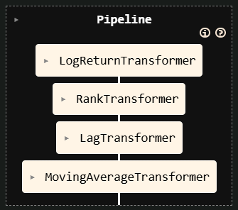
Explanation:

• set_config(enable_metadata_routing=True) turns on scikit-learn's metadata routing.
• set_transform_request(metadata_name=True) on each transformer tells the pipeline that this transformer expects metadata_name (e.g., date_series).
• When pipeline.fit_transform(X, date_series=dates, ticker_series=tickers) is called:
  • The date_series is automatically passed to RankTransformer.
  • The ticker_series is automatically passed to LagTransformer, MovingAverageTransformer, and LogReturnTransformer.
  • The output of LogReturnTransformer is passed to RankTransformer
  • The output of RankTransformer is passed to LagTransformer
  • The output of LagTransformer is passed to MovingAverageTransformer

This allows for complex data transformations where different steps require different auxiliary information, all managed cleanly by the pipeline.

# Now you can use this pipeline with your data
feature_names = ['open', 'high', 'low', 'close']
transformed_df = feature_pipeline.fit_transform(
    df_polars[feature_names],
    date_series=df_polars["date"],
    ticker_series=df_polars["ticker"],
)

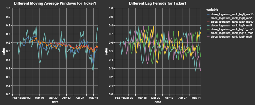
We can take a closer look at a sample output for a single ticker and for a single initial feature. This clearly shows how the close price for a cross-sectional dataset is transformed into a log return, ranked (between 0 and 1) by date, and smoothed (moving average windows) by ticker:

End-to-End Pipeline with an Estimator

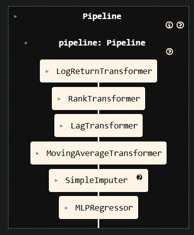
The previous "Advanced Pipeline" example constructed only the feature engineering part of a workflow. Thanks to Centimators' Keras-backed estimators you can seamlessly append a model as the final step and train everything through a single fit call.

from sklearn.impute import SimpleImputer
from centimators.model_estimators import MLPRegressor


lag_windows = [0, 5, 10, 15]
ma_windows = [5, 10, 20, 40]

mlp_pipeline = make_pipeline(
    # Start with the existing feature pipeline
    feature_pipeline,
    # Replace NaNs created by lagging with a constant value
    SimpleImputer(strategy="constant", fill_value=0.5).set_output(transform="pandas"),
    # Train a neural network in-place
    MLPRegressor().set_fit_request(epochs=True),
)

feature_names = ["open", "high", "low", "close"]

mlp_pipeline.fit(
    df_pl[feature_names],
    df_pl["target"],
    date_series=df_pl["date"],
    ticker_series=df_pl["ticker"],
    epochs=5,
)

Just as before, scikit-learn's metadata routing ensures that auxiliary inputs (date_series, ticker_series, epochs) are forwarded only to the steps that explicitly requested them.