pyhrp

A recursive implementation of the Hierarchical Risk Parity (HRP) approach by Marcos Lopez de Prado. We take advantage of the scipy.cluster.hierarchy package.

Motivation

Mean-variance optimisation is often unstable in practice because small estimation errors in expected returns can lead to large and concentrated weight shifts. Hierarchical Risk Parity avoids explicit return forecasting and instead allocates risk recursively along a clustering tree built from asset co-movement. By grouping correlated assets before sizing positions, HRP tends to distribute risk across more independent sources, which can improve diversification. In short, HRP keeps the intuition of risk budgeting while adding structure from correlation-based clustering.

Method comparison

The method argument controls how the first clustering tree is built:

Linkage method	When to use it
ward	Default choice when you want compact, variance-minimizing clusters and generally stable, balanced trees.
single	Useful when preserving nearest-neighbour chains matters (can create long, unbalanced trees on noisy data).
average	Middle ground between single and complete when you want moderate sensitivity to pairwise distances.
complete	Prefer when you want tighter, diameter-controlled clusters and to avoid chaining effects from single.

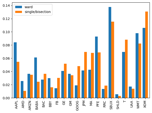
Setting bisection=True keeps the leaf order induced by the chosen linkage method, then rebuilds the tree by repeatedly splitting that ordered list in half. This often produces a more balanced hierarchy than the raw linkage tree and matches the bisection-style construction discussed in HRP literature.

Here's a simple example

import polars as pl
from pyhrp.hrp import build_tree, compute_cov, compute_corr
from pyhrp.algos import risk_parity

prices = pl.read_csv("tests/resources/stock_prices.csv", try_parse_dates=True).drop("date")

returns = prices.select(pl.all().pct_change()).drop_nulls().fill_null(0.0)
cov = compute_cov(returns)
cor = compute_corr(returns)

# Compute the dendrogram based on the correlation matrix and Ward's metric
dendrogram = build_tree(cor, method='ward')
dendrogram.plot()

# Compute the weights on the dendrogram
root = risk_parity(root=dendrogram.root, cov=cov)
root.portfolio.plot(names=dendrogram.names)

For your convenience you can bypass the construction of the covariance and correlation matrix, and the construction of the dendrogram.

from pyhrp.hrp import hrp
root = hrp(prices=prices, method="ward", bisection=False)

Interpreting results

The hrp() function returns a Cluster node (the tree root), not a plain weight series. You can navigate the hierarchy directly via root.left and root.right to inspect how the recursive allocation split risk at each branch. To get a flat asset-to-weight mapping for downstream use, access root.portfolio.weights.

weights = root.portfolio.weights
variance = root.portfolio.variance(cov)

# You can drill deeper into the tree
left = root.left
right = root.right

The comparison image above is generated from code in book/marimo/demo.py. Regenerate it with:

uv run --with kaleido book/marimo/demo.py

uv

Starting with

make install

will install uv and create the virtual environment defined in pyproject.toml and locked in uv.lock.

marimo

We install marimo on the fly within the aforementioned virtual environment. Executing

make marimo

will install and start marimo.