TypeToken API
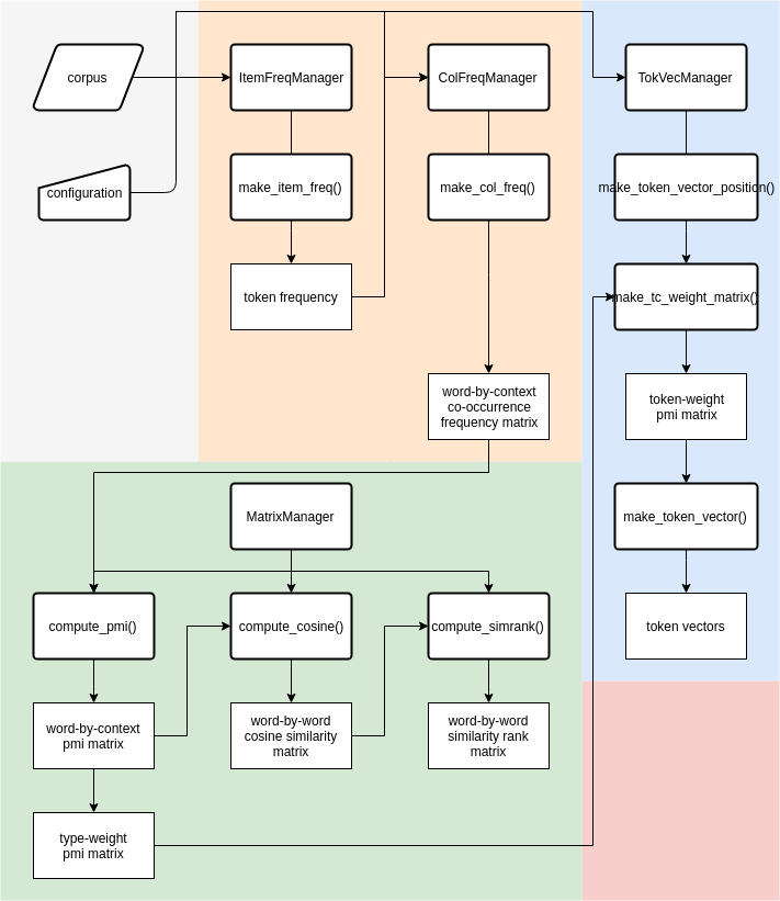
As the flowchart 1 below shows, the typeToken workflow is subdivided in three parts: one for generating token/type frequency dictionaries, one for creating the type vectors and one for creating token vectors. The token-level workflow partially relies on output from the type-level workflow. Therefore, I will first discuss the workflow to create type-level word spaces and then the workflow for the token-level. Since some functions are shared between the two workflows, I will occasionally refer back to the type-level discussion in the section on the token-level workflow.
This section describes how to build a type-level Word Space. Code examples will be displayed in boxes as if executed in an interactive session. As a convention, we use $ as the prompt symbol for Linux command line, and >>> as the prompt symbol for python sessions.
The typetoken code is in the directory /home/aardvark/code/typetokenQLVL/ (using typetokenQLVL to differentiate it from the original typeToken directory).
$ ls /home/aardvark/code
tokenclouds typeToken typetokenQLVL
Since many required packages such as scipy have not been installed for the default python on r2d2 and robin servers, you can use the python provided by a python virtual environment. Python virtual environments are provided in /home/aardvark/tools/VENV directory. This directory includes two virtual environments respectively for Python 2 and 3. The following code box shows the procedure to use. First you should activate the environment by source command. And then there would be an indicator (PY_VENV) before your command line. This means you are now working in a python virtual environment. The python you used here is different with the default python of server. To leave this virtual environment, you can use command deactivate. The Python 3 version is preferred.
$ source /home/aardvark/tools/VENV/PY_VENV/bin/activate
(PY_VENV) [...]$ python --version
Python 2.7.13
(PY_VENV) [...]$ deactivate
[...]$ python --version
Python 2.6.6
$ source /home/aardvark/tools/VENV/PY3_VENV/bin/activate
(PY3_VENV) [...]$ python --version
Python 3.6.4
(PY3_VENV) [...]$ deactivate
[...]$ which python
/usr/bin/python
After activating the virtual environment, we can also use commands to start Jupyter notebook on this remote server and use it on your local computer. There is another small tutorial on how to use Jupyter notebook on a remote server. And there are also ipython snippets files about how to use the typetoken model in the folder /home/aardvark/code/typetokenQLVL/snippets.
To run your own code, you can create a new ipython file or copy a snippets.ipynb file in your own folder, use Python console to code line by line, or create a new python file or copy a snippets.py file. All the codes presented below could be executed the same on Jupyter notebook as on Python.
Use the python of virtual environment to go to python interactive console. The following code adds your typetokenQLVL package to the system paths. The path is the father directory of the real typetoken package. Then we can import modules from the typetoken package.
>>> import sys
>>> sys.path.append("/home/aardvark/code/typetokenQLVL")
The "config.ini" file in the package consists of the default parameter settings, including basic information on the format of a corpus. In your real research, some parameter settings should be modified. A good way to change settings is to copy the "config.ini" file to your working directory and modify it based on your requirements. You should change those settings in the new "config.ini" file if they are different from the default settings and remove other redundant parameters:
file-encoding=utf-8
As mentioned before, the default character encoding for files is UTF8.
word-line-machine=([^\t]+)\t([^\t]+)\t([^\t]+)
The default format of a corpus file is 1 word per line. A word-line consists of three tab-delimited columns in the format wordform+TAB+part-of-speech+TAB+lemma. This three column format is set in the configuration file under the key "word-line-machine" through a regular expression. If the word-lines in your corpus are different, for example with four columns and whitespace-separated values (e.g. linenumber + SPACE + wordform + SPACE + part-of-speech + SPACE + lemma), then you can reset the regular expression in the settings dictionary accordingly (please do keep the round brackets as grouping feature for extracting the column values later on):
word-line-machine=(\S+)\s(\S+)\s(\S+)\s(\S+)
The corpus can also have other, non-word lines (e.g. sentence or article delimiters), but they CANNOT have the same format as a word-line.
separator-line-machine=</artikel>
One of the other line types in a corpus file can be a separator line, that is a hard boundary for any context window used by the distributional models. The default format of a separator line is < /artikel > (derived from the article boundaries in our Dutch news paper corpora), but again, this can be re-set based on your corpus format.
get-node=3,2
The default format for a target word (or node in Corpus Linguistic parlance) is lemma+/+part-of-speech. This information is retrieved from the columns on the word-line by the lambda-function, stored in settings["get-node"], which accesses the match-object created by matching the regular expression stored in settings["word-line-machine"] with a word-line: In the get-node setting 3 refers to the 3rd column with the lemma and 2 is the 2nd column with the part-of-speech. Again, this can be re-set based on your corpus’ word-line format and corresponding regular expression stored in settings["word-line-machine"]
get-colloc=3,2
The default format for a context word (or collocate in Corpus Linguistic parlance) is also lemma+/+part-of-speech.
You should also set in the configuration file your corpus-path and output-path. The corpus-path is the directory where your corpus file is stored. The output-path is the directory where you want to put your output data.
corpus-path=/home/aardvark/corp/en/BROWN_family/Brown_wpr-art
output-path=/path/to/your/output
Of course you can change the values in your code and this would be a better choice when you only have a few settings to change. However, when you have to change many settings, it is better for you to set them correctly in your configuration file before you start coding. After modifying the settings in "config.ini" file, you can import the ConfigLoader class and use it to load the default configuration file. Then, given your configuration file, the method updateConfig updates the default settings.
>>> from typetoken.Config import ConfigLoader
>>> default_conf = '/home/aardvark/code/typetokenQLVL/typetoken/config.ini'
>>> conf = ConfigLoader(default_conf)
>>> new_conf = '/path/of/your/config.ini'
>>> settings = conf.updateConfig(new_conf)
>>> corpus_name = 'Brown_wpr-art'
>>> corpus_path = settings['corpus-path']
>>> output_path = settings['output-path']
The corpus_name variable is a name for your corpus or your project to include at the beginning of the filenames that you will generate. You can set it different to the real name of the corpus. The corpus_path is the directory of corpus. For example, if your corpus file directory is "/home/tao/corpus/en/BROWN_family/Brown_wpr-art", then the corpus_path should be that and the corpus_name could be Brown_wpr-art or Brown, etc.
Before we start collecting co-occurrence data, we generate a simple frequency list from our corpus. If you already have a fnames file for all selected file names of corpus files, you can provide it for make_item_freq() method. Otherwise the method will process all files in corpus directory. It doesn't matter if the corpus directory has other directories inside.
>>> from typetoken.Manager import ItemFreqManager
>>> form = 'node'
>>> fnames = "/home/enzocxt/Projects/QLVL/typetoken_workdir/typetokenQLVL/test_data/Brown_wpr-art/Brown_wpr-art.fnames"
>>> ifman = ItemFreqManager(corpus_name, settings)
>>> freqDict = ifman.make_item_freq(fnames=fnames, form=form)
Making item frequency dict: Brown_wpr-art (node frequency)
  corpus: 100%|███████████████████████████████████████| 500/500 [00:25<00:00, 19.34file/s]

************************************
function      = make_item_freq
  arguments = [<class 'typetoken.Manager.ItemFreqManager'>] {'fnames': '/home/tao/test_typetoken/Brown_wpr-art.fnames', 'form': 'node'}
  time      = 26.067284 sec
************************************
The function will make a list of all word types that occurred in the corpus. Different parameter settings allow the word types to be counted on the word-form or lemma level, and with or without part-of-speech disambiguation. The output file has the extensions .nodefreq. As you can see above, the standard output first shows the progress bar of the process and then, after the processe is completed, it shows the time cost of the process including the function name and its arguments.
You could also print information about this frequency dict.
>>> freqDict.describe()
               freq
count  57737.000000
mean      18.805584
std      446.208395
min        1.000000
25%        1.000000
50%        2.000000
75%        5.000000
max    69735.000000
Write the item frequency list to file in json format.
>>> filename = "/path/to/output/file"
>>> freqDict.save(filename)
The output json file looks like:
{
    "Tarzan/NP0": 4,
    ...
}
Later on, if needed, you can reload the frequency dict with the .load() method:
>>> from typetoken.Dict import FrequencyDict
>>> freqDict = FrequencyDict.load(filename)To generate the co-occurrence matrix you need target words and context words. The FrequencyDict class provides methods for filtering the frequency dict, for example matching the nodes with a regular expression or setting a threshold for frequency. You can also select the most/least frequent nodes by slicing (the order of the dictionary is from most frequent to least frequent). If you select part of speech as well, don't forget to check if in your corpus it has lowercase or uppercase. The example below assumes uppercase.
>>> target_words_fname = "{}/{}.NounsLowercase.minfreq10.nodefreq".format(output_path, corpus_name)
>>> fd1 = freqDict[freqDict.match('item', '^[a-z][a-z]+/N.*'), freqDict.freq >= 10]
>>> fd1.save(target_words_fname)
>>> context_words_fname = "{}/{}.minfreq10.without50mostfreq.nodefreq".format(output_path, corpus_name)
>>> fd2 = freqDict[freqDict.match('item', '^[a-zA-Z][a-z]+'), freqDict.freq >= 10]
>>> fd2 = fd2[50:]
>>> fd2.save(context_words_fname)
>>> top5k = "{}/{}.top5k.without50mostfreq.nodefreq".format(output_path, corpus_name)
>>> fd3 = fd2[:5000]
>>> fd3.save(top5k)
To think about when filtering -- about the size of the dictionaries and matrices:
The length of these files will determine the size of the matrices you generate along the workflow. Their content will define the information available in them. For the collocation matrix, you will need two files (which could of course be the same): one for target words (rows of the collocation matrix) and one for context words (columns of the collocation matrix). If the length of the target words file is A and the length of context words is B, the size of the collocation matrix will be AxB. That said:
- When you generate a cosine similarity matrix, it will compare the rows, that is, the target words. The size of the cosine similarity matrix will then be AxA.
- When you get the token level matrix, you will use the target words as context features in the first step, but the features of the final matrix will be the context words. If you have C tokens, then, you will first generate a matrix of CxA and then end up with a matrix of CxB (B-dimensional token vectors). The cosine similarity matrix at vector level will be CxC.
If your matrices are too large, the computing time might be too long (even if it's not, the saving time will). It would seem that the time it takes to generate the collocation matrix depends on the number of rows more than the columns (a 10kx5k matrix took me almost an hour, a 5kx10k matrix took me half). But the longer your vectors are, the more features you can compare. You might want to take this into account while filtering the frequency wordlists.
The first step in building a type-by-context frequency matrix is to collect all co-occurrence frequencies between target words and context words from your corpus files, given a specific context window.
The parameters that you may need to change in config.ini file are:
- corpus format: in word-line-machine and separator-line-machine
- window size: values of left-span and right-span
- word format: values of get-colloc and get-node
>>> from typetoken.Manager import ColFreqManager
>>> from typetoken.Dict import CollocDict
>>> wordDict = CollocDict.load(target_words_fname, encoding=settings['file-encoding'])
>>> contextDict = CollocDict.load(context_words_fname, encoding=settings['file-encoding'])
>>> cfman = ColFreqManager(corpus_name, settings, wordDict=wordDict, contextDict=contextDict)
>>> freqMTX = cfman.make_col_freq()
Making col frequency matrix: BrownNouns
  corpus: 100%|███████████████████████████████████████| 501/501 [00:50<00:00,  9.82file/s]
Building sparse matrix from python dict of dict...
  Rows: 3752, cols: 9022
  Done... Num of data: 1131186

************************************
function    = make_col_freq
  arguments = [<class 'Manager.ColFreqManager'>] {}
  time      = 53.995048 sec
************************************
The method make_col_freq(), returns a wordtype-by-contextfeature matrix with as rows the word types, as the columns the context features, and as the cells the raw co-occurrence frequencies between wordtypes and contextfeatures. The wordDict and contextDict were provided for row and column words. The sorted dicts are stored in the rowDict and colDict attributes of this matrix object freqMTX. As a default, the function will include ALL the wordtype-contextfeature pairs.
The function will treat all different word types as possible target or context words and will record all co-occurrences in a dict attribute named matrix of this cfman object. Then inside the method make_col_freq(), the method make_WCMatrix of cfman is executed to create a matrix object. You can also show the description information of the matrix.
>>> freqMTX.describe()
********Matrix Description********
matrix shape:	3752 X 9022
matrix format:	freq
is sparse:	True
num of eles:	1131186
density:	3.34%
**********************************
By the following method, you can save the matrix to a file with filename that you provide or is automatically generated. The wordtype-contextfeatures matrix is a WCMatrix matrix. The auto generated file name would be "{output_path}/{corpus_name}.wcmx.{fmt}.json" with fmt "freq" (for wordtype-by-contextfeature frequency matrix saved by json format).
>>> freqMTX.save()
Saving CSR sparse matrix to file...
/home/tao/workdir/Brown_wpr-art/BrownNouns.wcmx.freq.jsonSince you're not expected to do everything in one day, you may want to generate a matrix at some point and load it later. There are classes for different formats of matrices. WCMatrix is for collocate frequency matrix and pmi matrix. WWMatrix is for row-wise cos similarity matrix and similarity rank matrix. CCMatrix is for column-wise cos similarity matrix and similarity rank matrix. And for the token level there are also TCMatrix (token-context position matrix) and TVMatrix (token vectors). To load these matrices, use the following codes (importing the corresponding class first).
>>> from typetoken.Matrix import WCMatrix
>>> filename = "/path/to/output/xxx.wcmx.freq.json"
>>> freqMTX = WCMatrix.load(filename, fmt='freq')
>>> filename = "/path/to/output/xxx.wcmx.pmi.json"
>>> pmiMTX = WCMatrix.load(filename, fmt='pmi')
>>> from typetoken.Matrix import WWMatrix
>>> meta_fname = "/path/to/output/xxx.wwmx.cos.meta"
>>> npy_fname = "/path/to/output/xxx.wwmx.cos.npy"
>>> cosMTX = WWMatrix.load(meta_fname, npy_fname, fmt='cos')
>>> from typetoken.Matrix import TCMatrix
>>> filename = "/path/to/output/xxx.tcmx.position.json"
>>> tcMTX = TCMatrix.load(filename, fmt='position')
>>> from typetoken.Matrix import TVMatrix
>>> filename = "/path/to/output/xxx.tvmx.pmi.json"
>>> tokvecs = TVMatrix.load(filename, fmt='pmi')
The same goes for the Frequency Dictionary, which will actually be needed later in the token level.
>>> from typetoken.Dict import FrequencyDict
>>> filename = "/path/to/output/xxx.nodefreq"
>>> freqDict = FrequencyDict.load(filename)There is a MatrixManager class which has methods for calculations. These methods are class methods of MatrixManager class, which means you can directly use these methods by class name. Except for printing out description information, you can directly print the matrix. The row ids and column ids are replaced by corresponding word types and context features.
The pmi matrix is the one that you'll reuse in the token level, both for weighting and as second co-occurrence matrix.
>>> from typetoken.Manager import MatrixManager
>>> pmiMTX = MatrixManager.compute_pmi(freqMTX)
>>> print(pmiMTX)
[3752, 9022]  that/DTQ  what/PNQ  no/DT0   &/CJC  its/PNP  say/VVD  than/CJS  ...
quote/NN0     -0.4540   0.9846    0.2122   0.4373     -1.2334  2.3517   -0.7945   ...
head/NN0      -0.6727   -0.5642   -0.5868  -0.6120    -0.3959  -0.4296  -0.2536   ...
time/NN0      -0.2061   0.0405    0.3019   -1.0683    -0.4562  -0.0931  -0.0052   ...
man/NN0       -0.1445   0.4057    0.5893   -0.5626    -0.8511  0.5751   0.0186    ...
formulum/NN0  -0.9514   -2.4306   -0.7100  3.4460     -0.7883  -3.5675  -0.3015   ...
year/NN2      0.0300    -0.5737   -0.7849  -2.5034    -0.2624  -0.4942  0.6849    ...
way/NN0       0.2361    0.2363    0.5706   -0.7126    0.2227   0.0927   -0.1604   ...
...           ...       ...       ...      ...        ...      ...      ...       ...
>>> filename = "{}/{}.BrownNouns.wcmx.pmi.json".format(output_path, corpus_name)
>>> pmiMTX.save(filename)
Saving matrix to file...
/home/tao/workdir/Brown_wpr-art/BrownNouns.wcmx.pmi.json
These matrices have the same format of default output filename.
/output-path/corpus_name.wcmx.freq.json: the wordtype-by-contextfeature frequency matrix
/output-path/corpus_name.wcmx.pmi.json: the wordtype-by-contextfeature PMI weighted matrix
/output-path/corpus_name.wwmx.cos.meta: the meta data file of the wordtype-by-wordtype cosine similarity matrix
/output-path/corpus_name.wwmx.cos.npy: the wordtype-by-wordtype cosine similarity matrix (numpy file)
/output-path/corpus_name.wwmx.simrank.meta: the meta data file of the wordtype-by-wordtype similarity rank matrix
/output-path/corpus_name.wwmx.simrank.npy: the wordtype-by-wordtype similarity rank matrix (numpy file)
The cosine similarity matrix is the one used to generate the clouds. So if you want a type level cloud, this is the one; if you want a token level cloud, you want to jump now to token level and then apply this method to the final product.
>>> cosMTX = MatrixManager.compute_cosine(pmiMTX)
>>> print(cosMTX)
[3752, 3752]  quote/NN0  head/NN0  time/NN0  man/NN0  formulum/NN0  year/NN2  way/NN0  ...
quote/NN0     1.0000     0.0653    0.2098    0.2766   -0.0447       0.0717    0.1884   ...
head/NN0      0.0653     1.0000    0.0757    0.0306   0.0791        0.1055    0.0124   ...
time/NN0      0.2098     0.0757    1.0000    0.2467   0.0462        0.2102    0.2215   ...
man/NN0       0.2766     0.0306    0.2467    1.0000   0.0238        0.1691    0.2368   ...
formulum/NN0  -0.0447    0.0791    0.0462    0.0238   1.0000        0.0491    0.0589   ...
year/NN2      0.0717     0.1055    0.2102    0.1691   0.0491        1.0000    0.1554   ...
way/NN0       0.1884     0.0124    0.2215    0.2368   0.0589        0.1554    1.0000   ...
...           ...        ...       ...       ...      ...           ...       ...      ...
>>> filename = "{}/{}.BrownNouns.wwmx.cos".format(output_path, corpus_name)
>>> cosMX.save(filename)
Saving matrix...
Stored in files:
	/home/tao/workdir/Brown_wpr-art/BrownNouns.wwmx.cos.meta
	/home/tao/workdir/Brown_wpr-art/BrownNouns.wwmx.cos.npy
There's an extra piece of code in the wiki, 'after the workflow', showing how to load this to R and get a matrix with row and column names.
Cosine similarity matrix and similarity rank matrix have similar operations as pmi matrix. I'm not yet sure what we would use the similarity rank matrix for.
>>> simrankMTX = MatrixManager.compute_simrank(cosMTX)
>>> print(simrankMTX)
[3752, 3752]  quote/NN0  head/NN0  time/NN0  man/NN0  formulum/NN0  year/NN2  way/NN0  ...
quote/NN0     1          84        4         2        2471          67        5        ...
head/NN0      27         1         18        123      16            9         317      ...
time/NN0      6          173       1         2        580           5         3        ...
man/NN0       2          1641      6         1        2002          28        7        ...
formulum/NN0  3748       232       455       828      1             427       344      ...
year/NN2      302        85        3         11       708           1         21       ...
way/NN0       12         3254      5         2        690           29        1        ...
...           ...        ...       ...       ...      ...           ...       ...      ...
>>> simrankMX.save()
Saving matrix...
Stored in files:
	/home/tao/workdir/Brown_wpr-art/BrownNouns.wwmx.simrank.meta
/home/tao/workdir/Brown_wpr-art/BrownNouns.wwmx.simrank.npyThe type of distributional semantic model used by QLVL on the token level is an adaptation of the approach by Schütze (1998). The model constructs a token vector by averaging over the type vectors of the context words around the target token. As a first step, we have to collect information about the context words that co-occur with specific occurrences (tokens) of a word. This token-by-context information will be stored in a boolean matrix which will then be the input for the averaging over context type vectors.
Firstly, generate a file that lists the types for which token information should be recorded. The file should be in json format. The json file stores a dict of type name and its frequency. You'll use some frequency dictionary to get the frequency data.
>>> from typetoken.Dict import FrequencyDict
>>> filename = "/path/to/your/output/xxx.nodefreq"
>>> freqDict = FrequencyDict.load(filename, encoding = settings[encoding])
>>> type_list = ['person/NN0', 'person/NN2', 'morning/NN0', 'morning/NN2', 'solution/NN0', 'solution/NN2']
>>> out_fname = "{}/{}.typeSelection.json".format(output_path, project_name)
>>> freqDict.make_type_file(type_list, out_fname)
The method make_type_file() could generate a json file based on a list of types whose token information should be recorded. It keeps the frequencies of these types. The type selection file looks like:
{
    "person/NNO": 175,
    "person/NN2": 119,
    ...
}
Optionally set the file name that lists the valid context words. As a default, ALL context words within the window will be taken into account. Note that the next step in the workflow assumes that type-level vectors are available for the context words (are part of the feature file).
>>> from typetoken.Manager import TokVecManager
>>> typeFile = '{}/{}.typeSelection.json'.format(output_path, corpus_name)
>>> featureFile = '{}/{}.NounsLowercase.minfreq10.nodefreq'.format(output_path, corpus_name)
>>> tvman = TokVecManager(corpus_name, settings, type_fname=typeFile, feature_fname=featureFile)
>>> tvman.make_token_context_position()
The function make_token_context_position records the context words that co-occur with a token in a specified window. For the position, the relative position to the target token is used, e.g. -1 for the first word to the left of the token. This position matrix is stored in tvman manager object. You can generate an encapsulated matrix object of this position values by function make_token_context_matrix. You can also save it to a file for later usage. The cell value is 0 if the token does not co-occur with the context feature and the position if the context feature does occur with the token.
>>> tcMTX = tvman.make_token_context_matrix()
>>> tcMTX.save()
Saving matrix to file:
/home/tao/workdir/Brown_wpr-art/BrownNouns.tcmx.position.json
Following Schütze (1998), we construct a token vector by taking the average of the context words’ type vectors. This results in a so-called second-order co-occurrence (SOCC) vector: a token is modelled by the co-occurrences of its own co-occurring words. This also means that we need a type-level word-by-contextfeature matrix (wcmx) for those words that we want to take into account as potential context words for the tokens. Now it also becomes clear why the rows of this type-level matrix need to correspond to the columns of the boolean token-by-context matrix: We will use the boolean values to know which context word vectors we need to average over. The most straightforward way of averaging is to do a pointwise addition of all context word vectors and then divide the vector by the total number of context words observed for the token. However, there are 2 parameters we can vary:
- the vector operation: Instead of pointwise addition, we can also per-form pointwise multiplication of the context vectors. (See Mitchell and Lapata (2010) for a comparison of addition and multiplication)
- weighting of context words: Instead of giving all context words equal weight, we can give a higher weight to more important context words.
For now we are adding, and weighting words based on the association strength with the type of the token.
Not all context words observed in a window around the token are equally informative for the token’s meaning. Say we have token of dog in the sentence While walking to work, the teacher saw a dog chasing a cat and barking at it. In this case, bark and cat are much more indicative of the meaning of dog than teacher or work. We want to increase the contribution of these words’ type vectors to the average vector. One measure of informativeness is the pointwise mutual information measure (PMI) we used in the type-level matrix. We therefore extract from the type-matrix the PMI values between all context words and the types, whose tokens we want to model (eventually, other association measures will be available). The context words are the rows in the type-level matrix.
>>> typeWeight_file = '{}/{}.wcmx.pmi.json'.format(output_path, corpus_name)
>>> twMTX = WCMatrix.load(typeWeight_file, fmt = 'pmi')
>>> twMTX = twMTX.transpose()
>>> from typetoken.Manager import TokVecManager
>>> tcWeightMTX = TokVecManager.make_tc_weight_matrix(tcMTX, twMTX)
The method make_tc_weight_matrix() takes the token context position matrix (tcMTX) and the transposed type-weight matrix (twMTX) as arguments. The columns of twMTX are the context features of tcMTX, and the types of the tokens we selected must be among the rows of this transposed twMTX. The number of rows of twMTX does not matter, because those that don't match the types of the tokens are simply ignored.
For each token in tcMTX, this method selects the type from the rows of twMTX and updates the value of each cell of the token's row with the corresponding value in the type's row of twMTX. The result is a matrix with the same size as tcMTX but weighted values (tcWeightMTX).
The rows of the second order co-occurrence matrix (soccMTX) should be the columns of tcMTX. Thus, the make_token_vector() method, which takes soccMTX and tcWeightMTX as arguments, multiplies these two matrices, and the result is a matrix with as many rows as tcWeightMTX and tcMTX (the tokens) and as many columns as soccMTX (the context words of the pmi matrix).
>>> soccMatrix_file = '{}/{}.wcmx.pmi.json'.format(output_path, corpus_name)
>>> soccMTX = WCMatrix.load(soccMatrix_file, fmt = 'pmi')
>>> tokvecs = TokVecManager.make_token_vector(soccMTX, tcWeightMTX)
>>> print(tokvecs)
[583, 9022]            that/DTQ  what/PNQ  no/DT0   &/CJC  its/PNP  say/VVD   than/CJS  ...
solution/NN2/J80/678   -0.0947   -0.5914   0.0915   -2.3793    0.5428   -3.8075   0.0010    ...
solution/NN2/J51/1966  0.2752    8.0538    6.0027   -3.1528    3.9740   5.3207    0.3070    ...
solution/NN2/J51/1744  0.6531    5.3588    0.7572   -4.9064    0.6550   -0.8103   4.4451    ...
solution/NN2/J47/422   4.0102    2.3170    5.7120   -11.4624   10.5593  -1.8972   9.0527    ...
solution/NN2/J37/1566  8.6344    -6.7005   -1.5710  -18.4661   -7.1649  -9.8780   2.0714    ...
solution/NN2/J18/2246  -1.7007   -8.1422   -0.6722  21.9267    -1.6415  -12.0352  -1.0886   ...
solution/NN2/J18/2216  -1.7412   -7.6107   -1.3890  22.7778    -1.2382  -11.9318  -1.7604   ...
...                    ...       ...       ...      ...        ...      ...       ...       ...
The size of a matrix is not very important when computing cosine similarity, but it is for saving the file. A token vector matrix with 12 thousand rows takes quite a while to save, so in this case it's useful to make a sample of the matrix and store that. The method sample on a TCMatrix or TVMatrix (e.g. tvsample = tokvecs.sample()) creates a random sample of 10% of the rows of the original matrix. That can be adjusted with the argument percent (default value 0.1).
This method can be either applied to a token level matrix before weighting, after weighting or even after interacting with the second cooccurrence matrix.
Finally, you get a cosine similarity matrix. Like explained above,
>>> from typetoken.Manager import MatrixManager
>>> tokvecCos = MatrixManager.compute_cosine(tokvecs)
To save the token level cosine similarity matrix, choose a name (if we have several for different subsets, we might want to add that information to the filename) without an extension, and feed it to the save() method.
>>> filename = '{}/{}.tvmx.cos'.format(output_path, corpus_name)
>>> tokvecCos.save(filename=filename)
Saving matrix...
Stored in files:
	/home/mariana/COHA-II/COHA.tvmx.cos.meta
	/home/mariana/COHA-II/COHA.tvmx.cos.npy